Adversarial Example Attacks

Saturday. November 16, 2019

For a while now, I’ve been meaning to experiment with generating adversarial examples for fooling CNN’s. Just this week I came across this blog post and the accompanying paper by Anish Athalye explaining how to generate adversarial examples in Tensorflow. What striked my attention the most was how similiar the implementation is to the Neural Style Transfer assignment in Andrew Ng’s Deep Learning course: instead of optimizing the CNN weights to minimize a cost function, we are updating the input image!

So what a better way to experiment generating my own adversarial examples than jumping right into it!

I will be using Google Collab to run the optimization task, as running it on my macbook’s CPU would take much longer. This post is a jupyter notebook so you can download it from my github here and run it with your own images.

Setup

I will start by installing Tensorflow 1.14.

!pip install tensorflow-gpu==1.14.0

Now I will mount my Google Drive so I can read and save files.

from google.colab import drive
drive.mount('/content/gdrive/', force_remount=True)

Now let’s download a MobileNetv2 model code and pretrained weights. I’ll be using MobileNetv2 because it is a lightweight model but the same algorithm used here could be used to synthetize adversarial examples for other more complex models.

!git clone https://github.com/tensorflow/models.git

checkpoint="mobilenet_v2_1.0_224.ckpt"
!wget https://storage.googleapis.com/mobilenet_v2/checkpoints/mobilenet_v2_1.0_224.tgz

!tar -xvf mobilenet_v2_1.0_224.tgz

# labels file
!wget https://gist.githubusercontent.com/d3rezz/20e7ab051578e1d80c3cd51402967048/raw/1addc22b63b0d35d747c9fa0677ed29d9eaf711c/imagenet_1001_labels.txt

Creating adversarial examples

For a given input image $x$ , the CNN computes a probability $P(y|x)$ for each possible label $y$ .

An adversarial example $\widehat{x}$ can then be computed by maximizing the log-likelihood of the target class $y_t$ .

$\begin{aligned} \max_{\widehat{x}} \quad& \log P(y_t|\widehat{x})\\ \textrm{s.t.} \quad & \left\|\widehat{x}-x\right\|_\infty < \epsilon \\ & \widehat{x} \in \[0,1\] \\ \end{aligned}$

The constraint $\left\|\widehat{x}-x\right\|_\infty < \epsilon$ is there to ensure the adversarial example doesn’t look too different from the original image. $\widehat{x} \in \[0,1\]$ just ensures we have a valid image by limiting the pixel values.

In order to make our adversarial example robust to a variety of transformations $T$ (ie. rotations, noise, translations), we want now to optimize $\mathbb{E}_{t \sim T} \log P(y_t|t(\widehat{x}))$ . This way we aim to produce an example that works over the entire distribution of $T$ .

Going over the original paper, I found it hard to wrap my head around the simplification made for computing the gradient of the expected value $\nabla \mathbb{E}_{t \sim T} \log P\left(\hat{y} \mid t(\hat{\mathbf{x}})\right) = \mathbb{E}_{t \sim T} \nabla \log P\left(\hat{y} \mid t(\hat{\mathbf{x}})\right)$ . Turns out this simplification can be made if the loss function is smooth and bounded, as explained in this stackoverflow post.

In practice, this can be implemented in Tensorflow by minizing the cross-entropy loss between a batch of our payload image with different random transformations sampled from $T$ and the target loss.

As some image transformation operations provided by Tensorflow only work for a single image at a time, instead of creating a batch of images, a single payload can be transformed and the loss computed multiple times and then averaged into a single loss.

It is important to note that if the the distribution of the transformations is very large, the adversarial input might not fool the network without increasing $\epsilon$ to allow for more significant changes in the image.

For more details on this algorithm, check out the original paper.

import tensorflow as tf
import sys
sys.path.append('/content/models/research/slim')
from nets.mobilenet import mobilenet_v2
import numpy as np
from PIL import Image
import matplotlib.pyplot as plt
%matplotlib inline

# define our inputs
trainable_input = tf.Variable(np.zeros((224, 224, 3)), dtype = tf.float32)
image_input = tf.placeholder(tf.float32, (224, 224, 3), name="image_input")
assign_op = tf.assign(trainable_input, image_input)  #this op should be called before the first gradient step

apply_transform = tf.placeholder(tf.bool, (), name="apply_transform")

target_class_input = tf.placeholder(tf.int32, (), name="target_class_input")
labels = tf.one_hot(target_class_input, 1001)

# clip image
epsilon = 5.0/255.0
lower_bound = image_input - epsilon
upper_bound = image_input + epsilon
clipped_input = tf.clip_by_value(tf.clip_by_value(trainable_input, lower_bound, upper_bound), 0, 1)

# Apply transformations we want to make the example robust against
num_samples = 10

def random_transform(im):
  
  #random scale
  new_dim = tf.random_uniform([], minval=200, maxval=224, dtype=tf.int32)
  transformed_im = tf.image.resize_images(im, (new_dim, new_dim))
  transformed_im = tf.image.resize_with_crop_or_pad(transformed_im, 224, 224)
  
  #random rotations up to 45º
  transformed_im = tf.contrib.image.rotate(transformed_im, tf.random_uniform((), minval=-np.pi/4, maxval=np.pi/4))
  
  # TODO apply other transformations here: noise, translations, mean shift...
  
  return transformed_im

average_loss = 0
for i in range(num_samples):
  # Apply random transformations
  transformed_input = tf.cond(apply_transform, lambda: random_transform(clipped_input), lambda: clipped_input)
  
  # MobileNetv2 preprocessing
  preprocessed_input = tf.expand_dims(transformed_input, 0)  #batch size = 1
  preprocessed_input = tf.subtract(tf.divide(preprocessed_input, 0.5), 1)
  with tf.contrib.slim.arg_scope(mobilenet_v2.training_scope(is_training=False)):
    logits, _ = mobilenet_v2.mobilenet(preprocessed_input, reuse=tf.AUTO_REUSE )
  probabilities = tf.nn.softmax(logits)
  
  # Loss for batch of transformed inputs
  loss = tf.nn.softmax_cross_entropy_with_logits(logits=logits, labels=[labels])
  average_loss += loss/num_samples

# Optimizer
optim_op = tf.train.GradientDescentOptimizer(0.1).minimize(average_loss, var_list=[trainable_input])

                                                                         
# For loading model
mb_vars = tf.get_collection(tf.GraphKeys.GLOBAL_VARIABLES, scope='MobilenetV2')
saver = tf.train.Saver(mb_vars)  

WARNING:tensorflow:From /content/models/research/slim/nets/mobilenet/mobilenet.py:364: The name tf.variable_scope is deprecated. Please use tf.compat.v1.variable_scope instead.

WARNING:tensorflow:From <ipython-input-9-8ac83bc4848f>:30: softmax_cross_entropy_with_logits (from tensorflow.python.ops.nn_ops) is deprecated and will be removed in a future version.
Instructions for updating:

Future major versions of TensorFlow will allow gradients to flow
into the labels input on backprop by default.

See `tf.nn.softmax_cross_entropy_with_logits_v2`.

WARNING:tensorflow:From /usr/local/lib/python3.6/dist-packages/tensorflow/python/ops/math_grad.py:1250: add_dispatch_support.<locals>.wrapper (from tensorflow.python.ops.array_ops) is deprecated and will be removed in a future version.
Instructions for updating:
Use tf.where in 2.0, which has the same broadcast rule as np.where

def square_crop(img, new_size=224):
  if img.width > img.height:
    new_height = new_size
    new_width = int(img.width * new_size/img.height)
  else:
    new_width = new_size
    new_height = int(img.height * new_size/img.width)
 
  img = img.resize((new_width, new_height))
  
  #center crop
  img = img.crop((int(new_width/2-new_size/2), int(new_height/2-new_size/2),int(new_width/2+new_size/2), int(new_height/2+new_size/2)))  # (left, upper, right, lower)
  
  return img

def get_label_string(id):
  with open("imagenet_1001_labels.txt", "r") as f:
    lines = f.readlines()
  return lines[id]

def get_label_id(label):
  lines = [line.rstrip() for line in open("imagenet_1001_labels.txt", "r")]
  return lines.index(label)

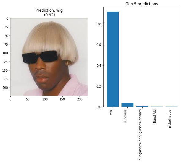
#Image to use for adversarial example
loaded_image = Image.open("/content/gdrive/My Drive/Colab Notebooks/images/tyler.jpg")
loaded_image = square_crop(loaded_image)
loaded_image = (np.asarray(loaded_image) / 255.0).astype(np.float32)[:,:,:3]

target_class = get_label_id("daisy")

def plot_prediction(image, probabilities, ax=None):
  prediction = np.argmax(probabilities)
  
  fig, (ax1, ax2) = plt.subplots(1, 2, figsize=(10, 6))
  ax1.imshow(image)
  ax1.title.set_text('Prediction: {} ({:.02f})'.format(get_label_string(int(prediction)), probabilities[prediction]))

  top_idx = list(probabilities.argsort()[-5:][::-1])
  
  top_probabilities = probabilities[top_idx]
  tick_label = [get_label_string(int(idx)) for idx in top_idx]
  ax2.bar(np.arange(5), probabilities[top_idx])
  ax2.set_xticks(np.arange(5))
  ax2.set_xticklabels(tick_label, rotation='vertical')
  ax2.title.set_text("Top 5 predictions")

# Start my tf session
sess = tf.Session()

# Load model weights
saver.restore(sess,  checkpoint)

WARNING:tensorflow:From /usr/local/lib/python3.6/dist-packages/tensorflow/python/training/saver.py:1276: checkpoint_exists (from tensorflow.python.training.checkpoint_management) is deprecated and will be removed in a future version.
Instructions for updating:
Use standard file APIs to check for files with this prefix.
INFO:tensorflow:Restoring parameters from mobilenet_v2_1.0_224.ckpt

I will take a photo of Tyler the Creator and see what it is originally classified as. Then, I will set the target_class as “daisy”, to make sure the network always classifoes him as a flower (boy!).

# Run prediction on input image
sess.run([assign_op], feed_dict={image_input: loaded_image})
payload, transformed_payload, p = sess.run([clipped_input, transformed_input, probabilities], feed_dict={image_input: loaded_image, apply_transform:False})
plot_prediction(transformed_payload, p[0,:])

png

# Create the adversarial example
steps = 300
sess.run([assign_op], feed_dict={image_input: loaded_image})
for i in range(steps):
  _, l = sess.run([optim_op, average_loss], feed_dict={image_input: loaded_image, target_class_input:target_class, apply_transform:True})
  if i%50==0:
    print("Step: {}\tLoss: {:.05f}".format(i, l[0]))

Step: 0	Loss: 8.84175
Step: 50	Loss: 0.11660
Step: 100	Loss: 0.04446
Step: 150	Loss: 0.03693
Step: 200	Loss: 0.01716
Step: 250	Loss: 0.01848

And here is our final payload image. The introduced changes are almost imperceptible!

# Get adversarial example (after it goes through clipping)
payload, transformed_payload, p = sess.run([clipped_input, transformed_input, probabilities], feed_dict={image_input: loaded_image, apply_transform:True})
fig, ax = plt.subplots()
ax.imshow(payload)

png

plt.imsave('/content/gdrive/My Drive/Colab Notebooks/output/adversarial_tyler.png', payload)

Let’s see how robust the adversarial example is to the transformations. Run the following cell a couple times to see the computed probabilities for different transforms of the adversarial example.

plot_prediction(transformed_payload, p[0,:])

png

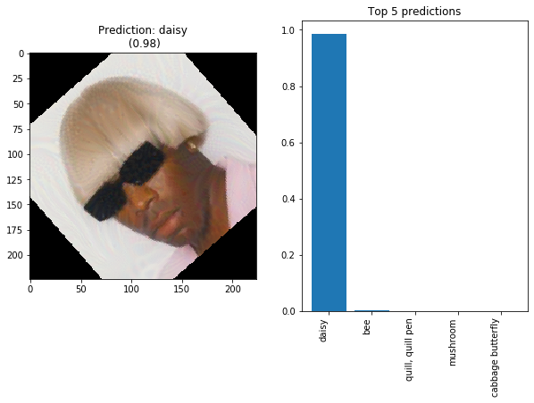
It’s a success!

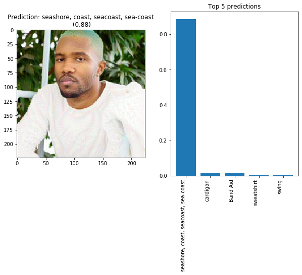
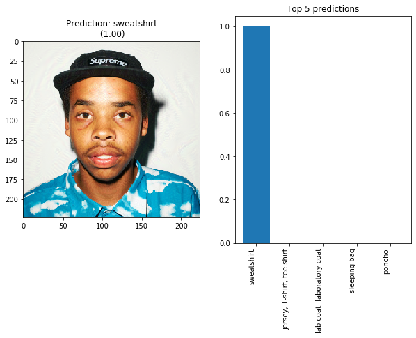
Bellow you can find a few more adversarial examples I’ve created before.

loaded_image = Image.open("/content/gdrive/My Drive/Colab Notebooks/output/adversarial_frank.png")
loaded_image = square_crop(loaded_image)
loaded_image = (np.asarray(loaded_image) / 255.0).astype(np.float32)[:,:,:3]
sess.run([assign_op], feed_dict={image_input: loaded_image})
payload, transformed_payload, p = sess.run([clipped_input, transformed_input, probabilities], feed_dict={image_input: loaded_image, apply_transform:False})
plot_prediction(payload, p[0,:])

png

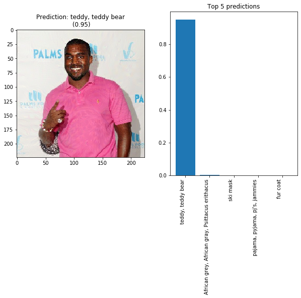
loaded_image = Image.open("/content/gdrive/My Drive/Colab Notebooks/output/adversarial_kanye.png")
loaded_image = square_crop(loaded_image)
loaded_image = (np.asarray(loaded_image) / 255.0).astype(np.float32)[:,:,:3]
sess.run([assign_op], feed_dict={image_input: loaded_image})
payload, transformed_payload, p = sess.run([clipped_input, transformed_input, probabilities], feed_dict={image_input: loaded_image, apply_transform:False})
plot_prediction(transformed_payload, p[0,:])

png

loaded_image = Image.open("/content/gdrive/My Drive/Colab Notebooks/output/adversarial_earl.png")
loaded_image = square_crop(loaded_image)
loaded_image = (np.asarray(loaded_image) / 255.0).astype(np.float32)[:,:,:3]
sess.run([assign_op], feed_dict={image_input: loaded_image})
payload, transformed_payload, p = sess.run([clipped_input, transformed_input, probabilities], feed_dict={image_input: loaded_image, apply_transform:False})
plot_prediction(transformed_payload, p[0,:])

png

Next time I revisit adversarial attacks, it would be great to experiment with black-box attacks (when we do not have access to the CNN model softmax outputs) as most CNN’s in the wild only return the top prediction label.

Printing the adversarial attacks and checking if they still hold up when taking a photo sounds fun too, however getting accurate colors with a printer might be a tricky step.

Adversarial Example Attacks

Setup

Creating adversarial examples

Related Posts