Softmax vs Triplet loss: Fashion-MNIST
Softmax vs Triplet loss: Fashion-MNIST
Since working on person re-identification (re-ID) during my master thesis, I’ve wanted to experiment with training models with using the triplet loss [1]
The triplet loss works by learning more robust feature representation of the data, where examples of the same class are close together on the feature space and examples belonging to different classes are further apart. It can be used for developing models for face identification [1], person re-identification [2], one-shot learning [3] or recommender systems as shown later in this post.
For this post, I will be using the Fashion-MNIST dataset [4], which contains images of 10 different items of clothing.
I will also experiment the tf.Estimator API to see if it reduces the amount of Tensorflow boilerplate code needed and helps making it more modular. Many available models use the tf.Estimator API so it should be useful to learn.
The code for this post is implemented using Tensorflow 1.13 and is available on my github.
Looking at the data
Let’s take a look at a 100 random examples from the Fashion-MNIST dataset.
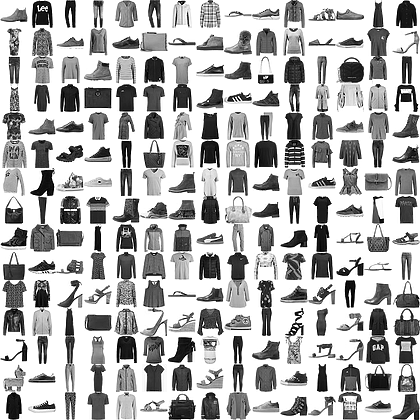
There are 10 different classes and images are labelled as follows:
| Label | Description |
|---|---|
| 0 | T-shirt/top |
| 1 | Trouser |
| 2 | Pullover |
| 3 | Dress |
| 4 | Coat |
| 5 | Sandal |
| 6 | Shirt |
| 7 | Sneaker |
| 8 | Bag |
| 9 | Ankle boot |
It is important to notice how shoes are almost always shown from the same side and all other clothing items are shown from the front.
Triplet loss
The triplet loss works by comparing 3 images at a time: an anchor, a positive (image of the same class) and a negative (image of a different class). It aims at minimizing the distance between the anchor and the positive while maximizing the distance from the anchor to the negative. The figure below should make it more clear:
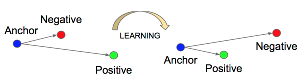
In contrast, the cross-entropy loss simply aims at learning a (non-linear) separation of the data. For certain applications, it might make sense to minimize the intra-class distance between embeddings while maximizing the inter-class distance, which is not directly optimized with the cross-entropy loss.
In mathematical notation, the triplet loss can be written as:
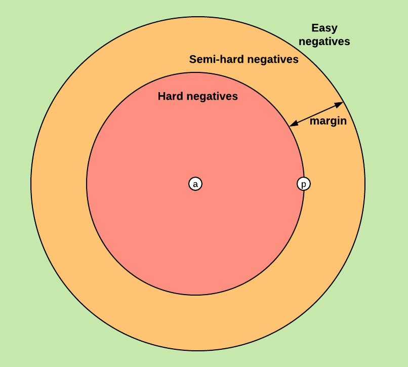
In practice, the margin value α sets how far the clusters of each class should be. For a more thorough explanation of the triplet loss, check [5].
Depending on how the negative is positioned in relation to the anchor and positive, it can be classified as:
[1] and [2] both recommend sampling K samples from P classes for selecting triplets during training. However, this is not easy to implement in an online fashion as required by the tf.Dataset API. Instead, I will use a batch size big enough to ensure valid triplets on each batch. Tensorflow already provides a function to compute semi-hard triplets in a batch and the corresponding loss tf.contrib.losses.metric_learning.triplet_semihard_loss. Nonetheless, I will be using Olivier Moindrot’s [5] implementations of the triplet loss function using all possible triplets and using only triplets with hard negatives in a batch, as they are beautifully implemented and vectorized.
The model
For computing the features of each image I will use a CNN with the following layers: 3 convolutional layers with 3x3 filters, followed by a global average pooling layer and lastly a fully connected layer to output the embedding. When training with cross-entropy loss, an additional fully connected layer is used to output the probabilities of the 10 classes.
The embedding_size is set to 64 for all experiments, meaning an embedding with 64 features is computed for each image.
with tf.variable_scope("model"):
    model = tf.layers.conv2d(images, 16, [3,3], strides=(2, 2), activation=tf.nn.relu)
    model = tf.layers.conv2d(model, 32, [3,3], strides=(1, 1), activation=tf.nn.relu)
    model = tf.layers.conv2d(model, 64, [3,3], strides=(2, 2), activation=tf.nn.relu)
    model = tf.reduce_mean(model, axis=[1,2])   # global avg pooling

    model = tf.layers.dense(model, params.embedding_size)   # do not add activation here

    # if using cross_entropy loss, add a FC layer to output the probability of each class
    if mode != tf.estimator.ModeKeys.PREDICT and params.loss == "cross_entropy":
        model = tf.layers.dense(model, params.num_classes)
I won’t be adding a L2-normalization layer after the embedding layer, as it does not seem necessary from [2]:
“We did not use a normalizing layer in any of our final experiments. For one, it does not dramatically regularize the network by reducing the available embedding space: the space spanned by all D-dimensional vector of fixed norm is still a D−1 - dimensional volume. Worse, an output-normalization layer can actually hide problems in the training, such as slowly collapsing or exploding embeddings.”
I will also skip the activation layer after computing the embeddings, as recommended in [5].
As the goal of this post is to experiment with the loss used for training, I won’t be focusing on developing a CNN for achieving high accuracy. Further improvements could be using achieved by using batch normalization, adding more convolutional layers and data augmentation.
Note: because items are almost always shown from the same side, not applying horizontal flips for augmentation shouldn’t hurt the performance too much.
Evaluation metrics
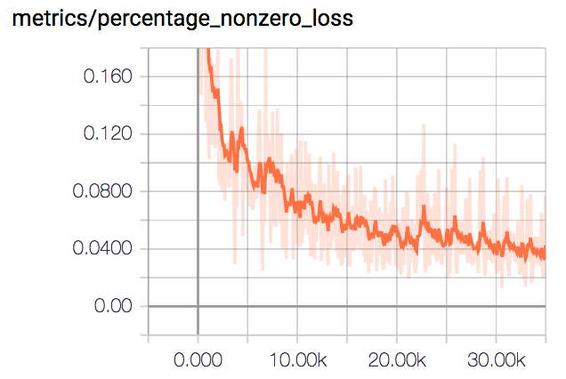
When training models using the triplet loss, there are several metrics we should keep track off. During training, the loss might stabilize. This does not mean the network has stopped learning. Instead, most of the triplets might be not valid and so they contribute 0 to the loss. So, we should keep an eye on percentage of non-zero losses in each batch (percentage_nonzero_loss) and if it is decreasing, then the model is still converging.
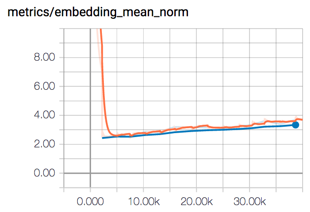
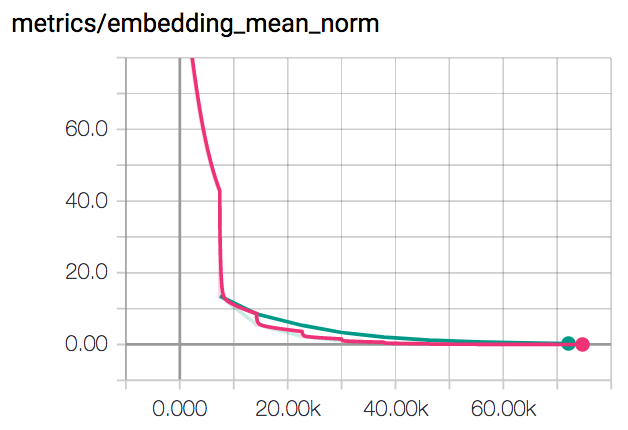
Another common issue is the network embeddings collapsing to a single point during training, i.e. due to a high learning rate. In other words, the embeddings are all becoming 0, and by keeping track of their mean norm(embedding_mean_norm) this situation can be easily identified.
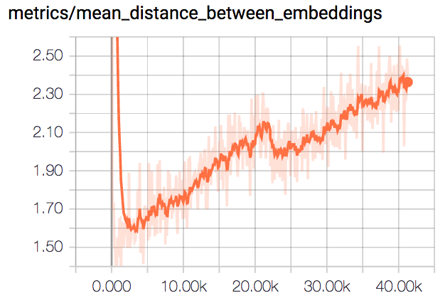
Finally, the mean_distance_between_embeddings serves as a proxy for the distance between embeddings of different classes and should increase during training.
When using the batch_hard loss, I will also keep track of the hardest_negative_distance and hardest_positive_distance.
For reporting metrics on Tensorboard with tf.Estimator during evaluation, a dictionary with all the relevant tf.metric needs to be created in addition to a tf.summary:
metrics = {}
embedding_mean_norm = tf.metrics.mean(tf.norm(embeddings, axis=1))
metrics["metrics/embedding_mean_norm"] = embedding_mean_norm
with tf.name_scope("metrics/"):
    tf.summary.scalar('embedding_mean_norm', embedding_mean_norm[1])
The metrics dictionary should then be passed to the EstimatorSpec constructor when evaluating:
if mode == tf.estimator.ModeKeys.EVAL:
        return tf.estimator.EstimatorSpec(mode, loss=loss, eval_metric_ops=metrics)
More details can be found in https://www.tensorflow.org/guide/custom_estimators.
During training, the loss and metrics reported are for a single batch. For evaluation, the loss and metrics are computed over all the validation examples.
Training
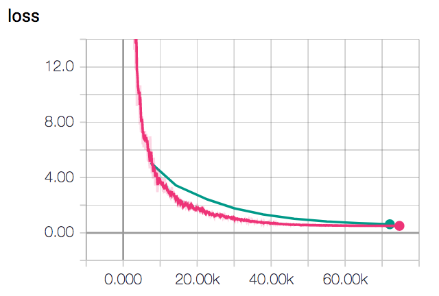
Below are the Tensorboard plots keeping track of the different metrics during training with the batch all methodology. The Adam optimizer was used, with a learning rate of 10-3. The orange line refers to training metrics, while the blue line referes to evaluation metrics. Smoothing of 0.6 was used.
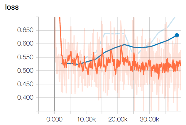
Until around 10k iterations, both losses converge together. After that, the evaluation loss starts to diverge slightly, increasing steeply after 25k iterations.
As mentioned in the previous section, while the training loss may stop decreasing after a certain value, this does not mean learning as stopped. As seen in the following plot of the percentage of nonzero losses (the percentage of valid triplets) just keeps decreasing, meaning weights keep being updated.
By looking at the embeddings_mean_norm plot, we can observe the embeddings haven’t all collapsed to the same point. The inter-class distance also increases as seen in the plot of mean_distance_between_embeddings.
I found training with the batch hard strategy much more instable. With a low learning rate of 10-6, the loss converged to 0.5, which is equal to the margin value.
By looking at the following plot of the mean of the norm of the embeddings, we can see they all collapsed to the same point, instead of getting further away of each other.
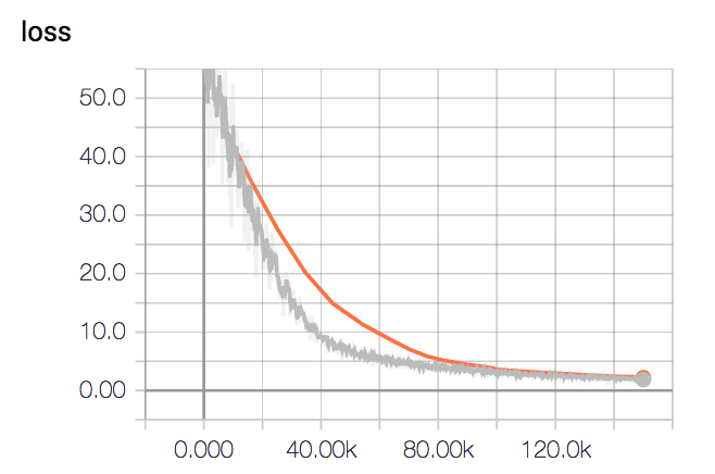
By lowering the learning rate to 10-7, computed embeddings don’t seem to collapse right away. However, the training loss (grey color in the plot below) converges very slowly, and even after 150k iterations it is still converging.
I found the following comment in [5] very insightful:
“My intuition is that the batch all strategy has more information so when you train from scratch with triplet loss, it will be easier at first. The batch hard strategy might be better when the network is already well trained or if you are fine-tuning pre-trained weights. One issue with batch hard is also that if your dataset is very noisy, it will focus on these noisy / mislabeled examples and not really learn.”
Visualizing the results
With the model training we can now compute the Euclidean distance between the embeddings of two images to infer how similar they are (sample code in query_distances.py):
A more useful visualization can be achieved with T-SNE by reducing the 64 features being computed for each example to 2 and plotting them. A more thorough description of the T-SNE algorithm can be found in https://distill.pub/2016/misread-tsne/, as well as useful tips and considerations.
The following T-SNE plots, were produced by computing the embeddings first and then creating a ProjectorConfig for visualizing in Tensorboard. The code can be found in visualize.py.
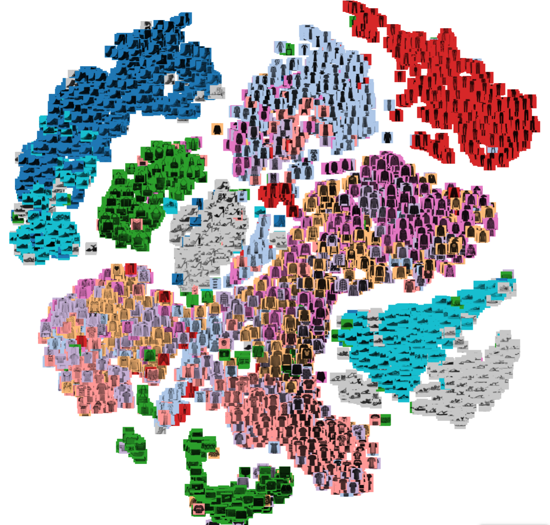 | 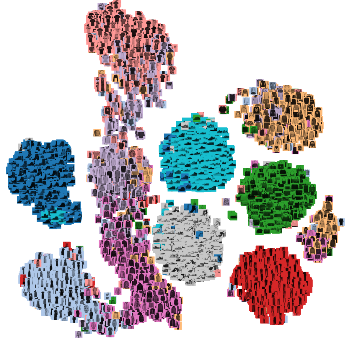 |
| Classification Loss | Triplet Loss (Batch All) |
While training with cross-entropy loss resulted in clusters that look separable, they almost overlap each other. On the other hand, training with triplet loss resulted in the extracted embeddings forming distinct clusters, containing a single type of clothing. There is some overlap on the clusters containing tshirts, shirts and pullovers. This is likely due to the very simple CNN architecture picked, which does have enough discriminating power.
Recommender System
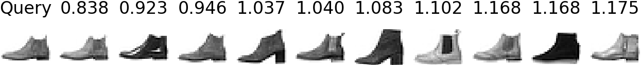
The triplet loss can be used to build a system to show recommendations to a customer shopping online.
Each item in the online store can be indexed by a feature extractor trained with triplet loss and stored in a database. Recommendations can then be suggested to the customer by retrieving the closest embeddings to the items currently being viewed by the customer.
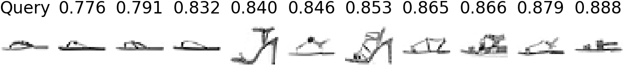
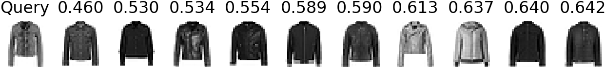
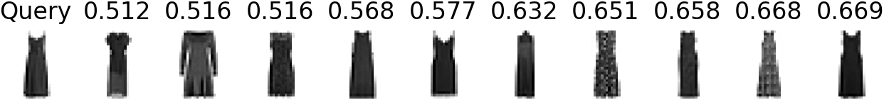
Below you can see samples queries to the clothes recommender system trained before. The first column shows the query item and the next columns show similar items ordered by their similarity. Example code is provided in recommender.py.
 |
 |
 |
 |
Conclusions
I hope this was as insightful to read as it was to write, and that you understood how useful the triplet loss is for training a model to compute embeddings. In the end, the triplet loss resulted in better separated classes, with examples belonging to the same class forming distinct clusters.
At first, I couldn’t wrap my head around how mining triplets online worked, but it proved much easier to implement and faster than precomputing the triplets.
Regarding the different triplet selection strategies, they need to be chosen according to the model and data: batch all results in more information to learn from when compared to the other strategies, so when training from scratch, there is less tendency for the embeddings to collapse to a single point and stopping the learning. It would be interesting to see if the same stands when training a more complex architecture in different dataset.
Also, the tf.Estimator API ended up being very intuitive to use and resulted in very modular and easy to read code. I will definitely be using it for loading and training my models from now on.
Further experiments
In future experiments, I would like to:
- Design a more powerful CNN for computing the embeddings and apply data augmentation;
- Train with semi-hard triplets and compare to the strategies used;
- Use a more problem specific metric to track training i.e rank-1 accuracy in a person re-identification setting.
References
[1] Schroff, Florian, Dmitry Kalenichenko, and James Philbin. “Facenet: A unified embedding for face recognition and clustering.” Proceedings of the IEEE conference on computer vision and pattern recognition. 2015
[2] Hermans, Alexander, Lucas Beyer, and Bastian Leibe. “In defense of the triplet loss for person re-identification.” arXiv preprint arXiv:1703.07737 (2017).
[3] Ng, Andrew, “Triplet Loss”, Deep Learning Specialization lecture notes, Coursera, www.coursera.org .
[4] https://github.com/zalandoresearch/fashion-mnist
[5] https://omoindrot.github.io/triplet-loss